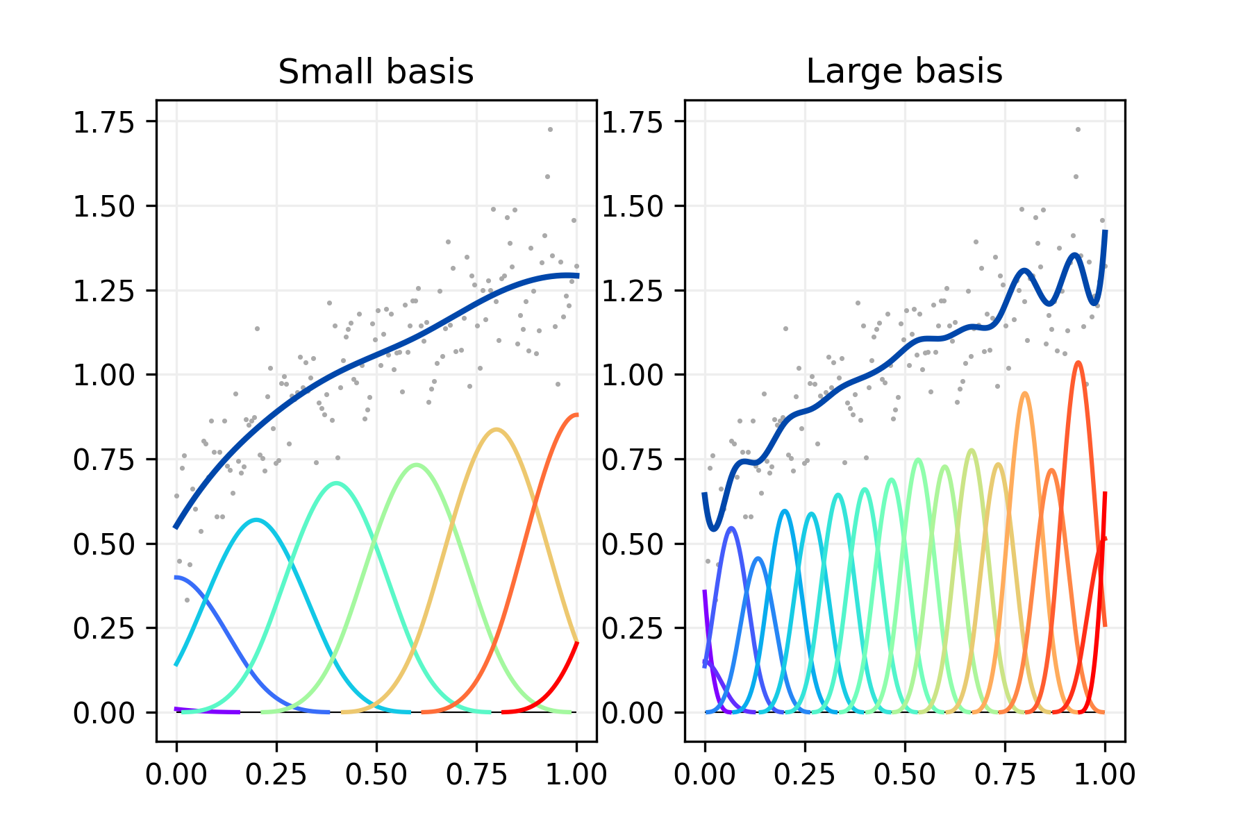
Illustration B-splines differing number of segments (simulated data)

import numpy as np
import matplotlib.pyplot as plt
import matplotlib.cm as cm

from pyspline.psplines import PSplines
from pyspline.basis import basis_bsplines


# Set RNG
rng = np.random.default_rng(42)


# Simulate data
n = 150
x = np.linspace(0, 1, n)
y = 0.3 + np.sin(1.2 * x + 0.3) + 0.15 * rng.normal(size=n)


# Make a matrix containing the small B-spline basis
ndx_s = 8
deg = 3
B_small = basis_bsplines(
    x, n_functions=ndx_s, degree=deg, domain_min=0, domain_max=1
)


# Make a matrix containing the large B-spline basis
ndx_l = 18
deg = 3
B_small = basis_bsplines(
    x, n_functions=ndx_l, degree=deg, domain_min=0, domain_max=1
)


# A basis for plotting the fit on the grid xg
ng = 500
xg = np.linspace(0, 1, ng)
Bg_small = basis_bsplines(
    xg, n_functions=ndx_s, degree=deg, domain_min=0, domain_max=1
)
Bg_large = basis_bsplines(
    xg, n_functions=ndx_l, degree=deg, domain_min=0, domain_max=1
)


# (Small) Estimate the coefficients and compute the fit on the grid
ps_small = PSplines(penalty=0, n_segments=(ndx_s - deg,), degree=(deg,))
ps_small.fit(X=x.reshape(-1, 1), y=y)
z_small = ps_small.predict(X=xg.reshape(-1, 1))


# (Large) Estimate the coefficients and compute the fit on the grid
ps_large = PSplines(penalty=0, n_segments=(ndx_l - deg,), degree=(deg,))
ps_large.fit(X=x.reshape(-1, 1), y=y)
z_large = ps_large.predict(X=xg.reshape(-1, 1))


# Make a matrix with B-splines scaled by coefficients
Bsc_small = np.diag(ps_small.beta_hat_) @ Bg_small
Bsc_small[Bsc_small < 1e-4] = np.nan

Bsc_large = np.diag(ps_large.beta_hat_) @ Bg_large
Bsc_large[Bsc_large < 1e-4] = np.nan


# Build the graph
fig = plt.figure(figsize=(6, 4), dpi=300)
axs = fig.subplots(1, 2, sharex=True)

axs[0].scatter(x, y, color="#AAAAAA", s=0.5, zorder=3)
axs[0].plot(xg, z_small, color="#0047AB", linewidth=2, zorder=6)

colors = iter(cm.rainbow(np.linspace(0, 1, ndx_s)))
for idx in np.arange(ndx_s):
    c = next(colors)
    axs[0].plot(xg, Bsc_small[idx], color=c, zorder=3)
axs[0].hlines(0, xmin=0, xmax=1, color="#000000", linewidth=0.5)
axs[0].grid(linestyle="-", color="#EEEEEE", zorder=0)
axs[0].set_title("Small basis")

axs[1].scatter(x, y, color="#AAAAAA", s=0.5, zorder=3)
axs[1].plot(xg, z_large, color="#0047AB", linewidth=2, zorder=6)

colors = iter(cm.rainbow(np.linspace(0, 1, ndx_l)))
for idx in np.arange(ndx_l):
    c = next(colors)
    axs[1].plot(xg, Bsc_large[idx], color=c, zorder=3)
axs[1].hlines(0, xmin=0, xmax=1, color="#000000", linewidth=0.5)
axs[1].grid(linestyle="-", color="#EEEEEE", zorder=0)
axs[1].set_title("Large basis")

plt.show()