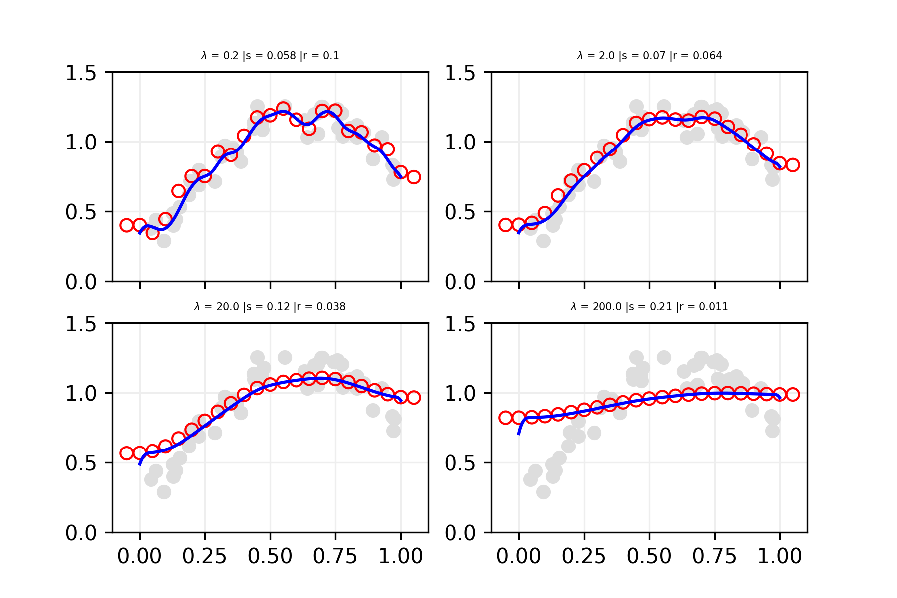
First order difference penalty in action with various tuning

import numpy as np
import matplotlib.pyplot as plt

from pyspline.psplines import PSplines


# Set RNG
rng = np.random.default_rng(42)


# Simulate data
m = 50
x = rng.uniform(0, 1, m)
y = np.sin(2.5 * x) + 0.1 * rng.normal(0, 1, m) + 0.2


# Large grid
nu = 200
xg = np.linspace(0, 1, nu)


# Basis parameters
nseg = 20
deg = 3
knots = (np.arange(1, nseg + deg + 1) - 2) / nseg


# Generate the plots
fig = plt.figure(figsize=(6, 4), dpi=300)
axs = fig.subplots(2, 2, sharex=True)

penalties = 2 * np.array([0.1, 1, 10, 100])
for idx, penalty in enumerate(penalties):
    ps = PSplines(
        penalty=(penalty,), n_segments=(nseg,), degree=(deg,), order_penalty=1
    )
    ps.fit(X=x.reshape(-1, 1), y=y)
    y_pred = ps.predict(X=xg.reshape(-1, 1))

    axs[idx // 2, idx % 2].scatter(
        knots, ps.beta_hat_, edgecolors="r", facecolors="none", zorder=4
    )
    axs[idx // 2, idx % 2].scatter(x, y, c="#DDDDDD", zorder=3)
    axs[idx // 2, idx % 2].plot(xg, y_pred, color="b", zorder=4)
    axs[idx // 2, idx % 2].grid(linestyle="-", color="#EEEEEE", zorder=0)
    axs[idx // 2, idx % 2].set_title(
        (
            f"$\lambda$ = {penalty} |"
            f"s = {ps.diagnostics_['residuals_std']:.2} |"
            f"r = {ps.diagnostics_['roughness']:.2}"
        ),
        size=5,
    )
    axs[idx // 2, idx % 2].set_ylim((0, 1.5))