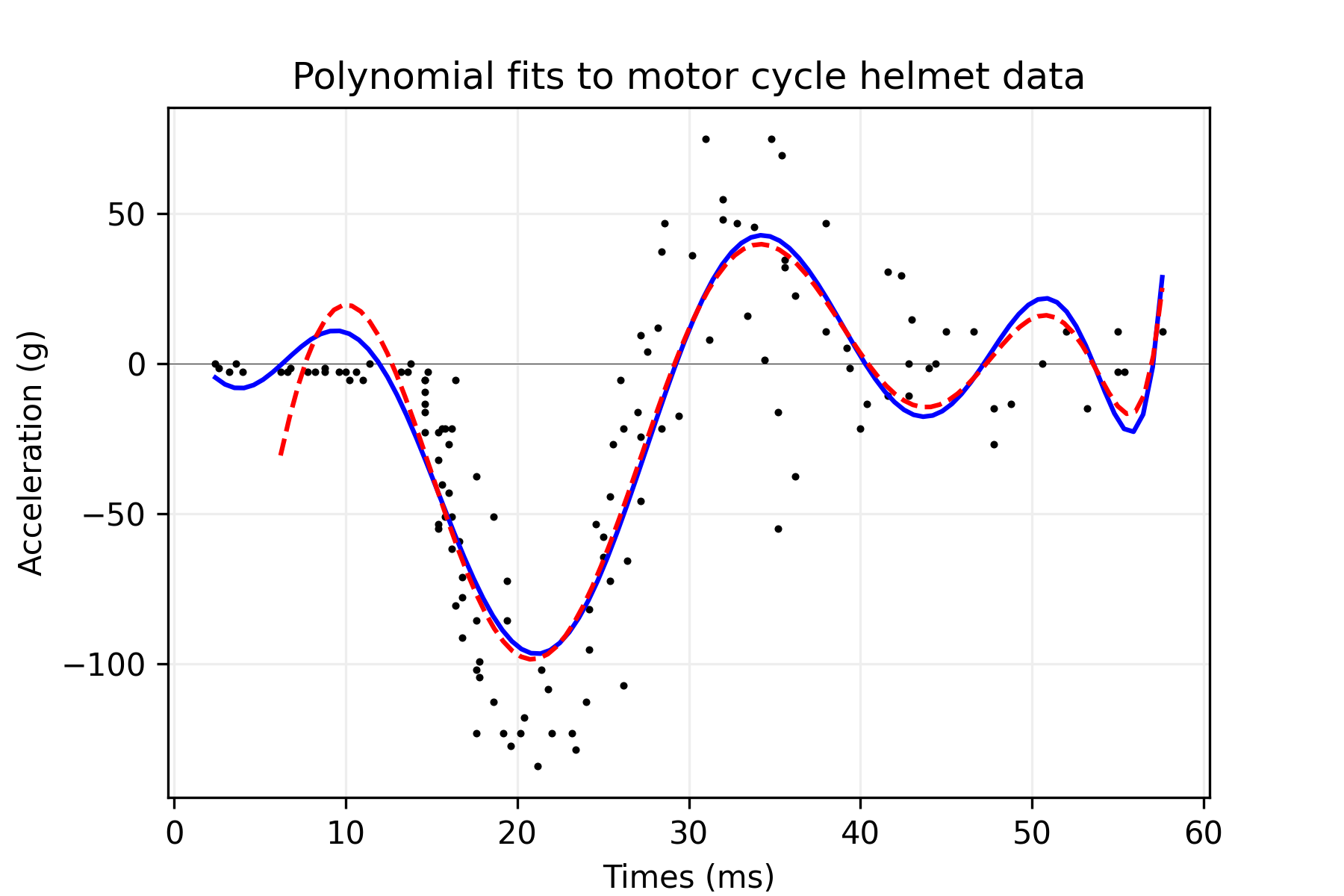
Polynomial fits with differing support (Motorcycle data)

import numpy as np
import matplotlib.pyplot as plt
import pandas as pd

from sklearn.linear_model import LinearRegression
from sklearn.pipeline import make_pipeline
from sklearn.preprocessing import PolynomialFeatures

# Get the data
data = pd.read_csv("../data/mcycle.csv").dropna()
times = data["times"].to_numpy()
accel = data["accel"].to_numpy()


def make_grid(x, n=100):
    return np.linspace(np.min(x), np.max(x), n)


# Fit based on all data
new_times = make_grid(times)
lm = make_pipeline(PolynomialFeatures(9), LinearRegression())
lm.fit(times.reshape(-1, 1), accel)
new_accel = lm.predict(new_times.reshape(-1, 1))


# Fit based on data where time is greater than 5ms
mask = times > 5
times_subset = times[mask]
accel_subset = accel[mask]
new_times_subset = make_grid(times_subset)
lm = make_pipeline(PolynomialFeatures(9), LinearRegression())
lm.fit(times_subset.reshape(-1, 1), accel_subset)
new_accel_subset = lm.predict(new_times_subset.reshape(-1, 1))


# Build the graph
plt.figure(figsize=(6, 4), dpi=300)
plt.scatter(times, accel, color="#000000", s=2, zorder=4)
plt.plot(new_times, new_accel, color="b", zorder=5)
plt.plot(
    new_times_subset, new_accel_subset, color="r", linestyle="dashed", zorder=5
)
plt.axhline(y=0, color="k", linewidth=0.2, zorder=3)

plt.title("Polynomial fits to motor cycle helmet data")
plt.xlabel("Times (ms)")
plt.ylabel("Acceleration (g)")
plt.grid(linestyle="-", color="#EEEEEE", zorder=0)
plt.show()