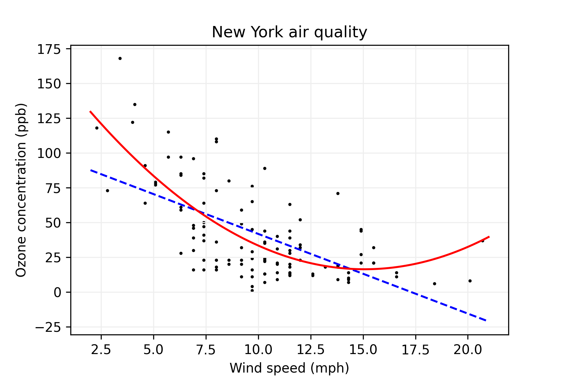
New York air quality data polynomial fits (air quality data)

import numpy as np
import matplotlib.pyplot as plt
import pandas as pd

from sklearn.linear_model import LinearRegression
from sklearn.pipeline import make_pipeline
from sklearn.preprocessing import PolynomialFeatures


# Get the data
data = pd.read_csv("../data/airquality.csv").dropna()
wind = data["Wind"].to_numpy()
ozone = data["Ozone"].to_numpy()


# Least squares linear
new_wind = np.arange(2, 21, 0.01)
lm = LinearRegression().fit(wind.reshape(-1, 1), ozone)
new_ozone_linear = lm.predict(new_wind.reshape(-1, 1))


# Least squares quadratic
new_wind = np.arange(2, 21, 0.01)
qm = make_pipeline(PolynomialFeatures(2), LinearRegression())
qm.fit(wind.reshape(-1, 1), ozone)
new_ozone_quadratic = qm.predict(new_wind.reshape(-1, 1))


# Build the graph
plt.figure(figsize=(6, 4), dpi=300)
plt.scatter(wind, ozone, color="#000000", s=2)
plt.plot(new_wind, new_ozone_linear, color="b", linestyle="dashed")
plt.plot(new_wind, new_ozone_quadratic, color="r")

plt.title("New York air quality")
plt.xlabel("Wind speed (mph)")
plt.ylabel("Ozone concentration (ppb)")
plt.grid(linestyle="-", color="#EEEEEE", zorder=0)
plt.show()